Chapter 6 Equations

6.1 Equation syntax

The syntax for equations is similar (but not identical) to LaTeX.

LaTeX code:

\begin{equation}
\label{eqn:friedman}
    \left(\dfrac{\dot{a}}{a}\right)^2 + \dfrac{kc^2}{a^2} = \dfrac{8\pi G}{3}\rho 
\end{equation}

Rmd code:

\begin{equation}
    \left(\dfrac{\dot{a}}{a}\right)^2 + \dfrac{kc^2}{a^2} = \dfrac{8\pi G}{3}\rho
(\#eq:friedman)
\end{equation}

\[\begin{equation} \left(\dfrac{\dot{a}}{a}\right)^2 + \dfrac{kc^2}{a^2} = \dfrac{8\pi G}{3}\rho \tag{6.1} \end{equation}\]

You can also use the latex

\begin{align}
...
\end{align}

format for equations. If you’re converting from LaTeX to markdown with pandoc it may convert equations to

\begin{aligned}
...
\end{aligned}

which also works.

LaTeX subequations and intertext

I haven’t been able to get subequations and intertext to work in bookdown. LaTeX equations of the form

\begin{subequations}\begin{align}
\vec{E} &= \left( x,t \right)
\intertext{and in 3 dimensional space as}
\vec{E} &= \left( x,y,z,t \right)
\end{align}\end{subequations}

should be written as separate equations with the text between written outside the equation environment, e.g.

\begin{align}
\vec{E} &= \left( x,t \right)
\end{align}
and in 3 dimensional space as
\begin{align}
\vec{E} &= \left( x,y,z,t \right)
\end{align}

6.2 Equation numbers and labels

The syntax for the maths is the same, but the labelling changes. To label and equation add

(\#eq:label)

just before end{equation}. Only equations with labels will be numbered. If you don’t want numbers then don’t label the equations, but numbers are helpful.

6.3 Cross referencing equations

The syntax for cross-referencing equations is similar to sections and figures, i.e.

Eqn. \@ref(eq:friedman) is the Friedman equation

will give “Eqn. (6.1) is the Friedman equation”.

6.4 Maths in captions

R markdown gets a bit finicky about maths/symbols in captions. You may need to use two backslashes to escape symbols in figure captions.

Example of a finicky caption:

```
{r echo=FALSE, gaussian, out.width='100%', fig.show='hold', fig.cap="Gaussian uncertainties. 
If we measure a value $x$ for a variable that has a true value $\\langle x \\rangle$ and
uncertainty $\\sigma$, there is a 68.3% probability that $x$ will be within 
$\\langle x \\rangle \\pm 1\\sigma$. There's a 95.4% probability of $x$ being within 
$\\langle x \\rangle \\pm 2\\sigma$, and 99.7% of $x$ being within  
$\\langle x \\rangle \\pm 3\\sigma$."}
knitr::include_graphics("Images/normal-curve.png")
```

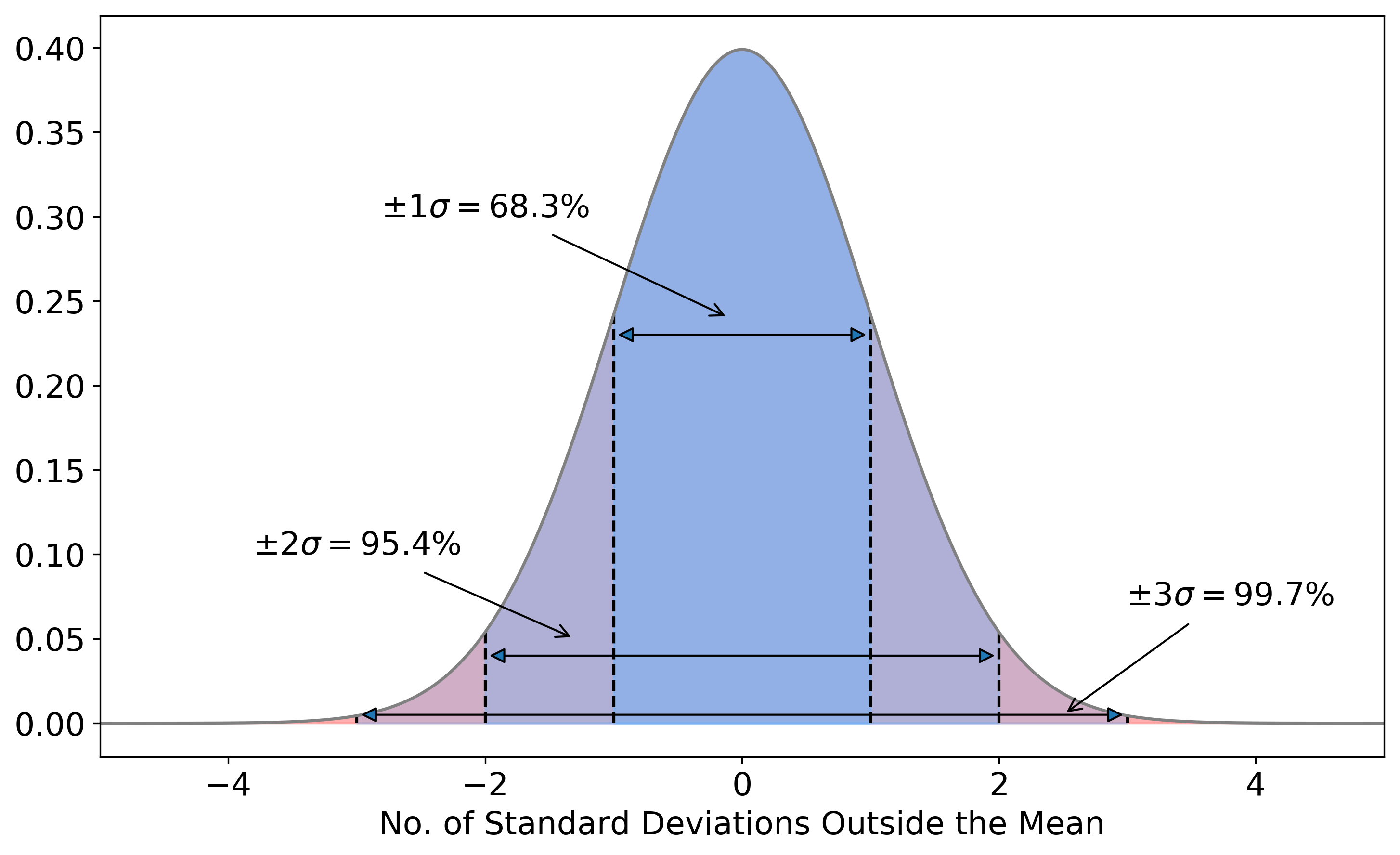
$Gaussian uncertainties. If we measure a value $x$ for a variable that has a true value $\langle x \rangle$ and uncertainty $\sigma$, there is a 68.3% probability that $x$ will be within $\langle x \rangle \pm 1\sigma$. There's a 95.4% probability of $x$ being within $\langle x \rangle \pm 2\sigma$, and 99.7% of $x$ being within $\langle x \rangle \pm 3\sigma$.$

Figure 6.1: Gaussian uncertainties. If we measure a value $x$ for a variable that has a true value $\langle x \rangle$ and uncertainty $\sigma$, there is a 68.3% probability that $x$ will be within $\langle x \rangle \pm 1\sigma$. There’s a 95.4% probability of $x$ being within $\langle x \rangle \pm 2\sigma$, and 99.7% of $x$ being within $\langle x \rangle \pm 3\sigma$.

6.5 Random tips

Angstrom symbol: Use $\unicode{x0212B}$ rather than $\AA$ to get $\unicode{x0212B}$. If you’re outputting to pdf via latex then you might get an error/missing symbol. This seems to be an annoying problem to fix in a way that works for pdf and html.